




What goes in a data lake dashboard in Metabase?
A data lake dashboard tracks ingestion volume by source, object and partition growth, the small-file problem, file-format mix, query-engine usage, and storage-tier costs. Where a warehouse dashboard watches queries and compute, this one watches the objects themselves — Metabase reads it all through the engines already on the lake, like Athena or Trino, over inventory and query-log rollups.
For: data platform engineers and lakehouse owners. Grain: one inventory snapshot per table per day, plus one row per engine query. Source: object-store inventory (S3 Inventory or equivalent), the catalog, and engine query logs.
What does a data lake dashboard look like?
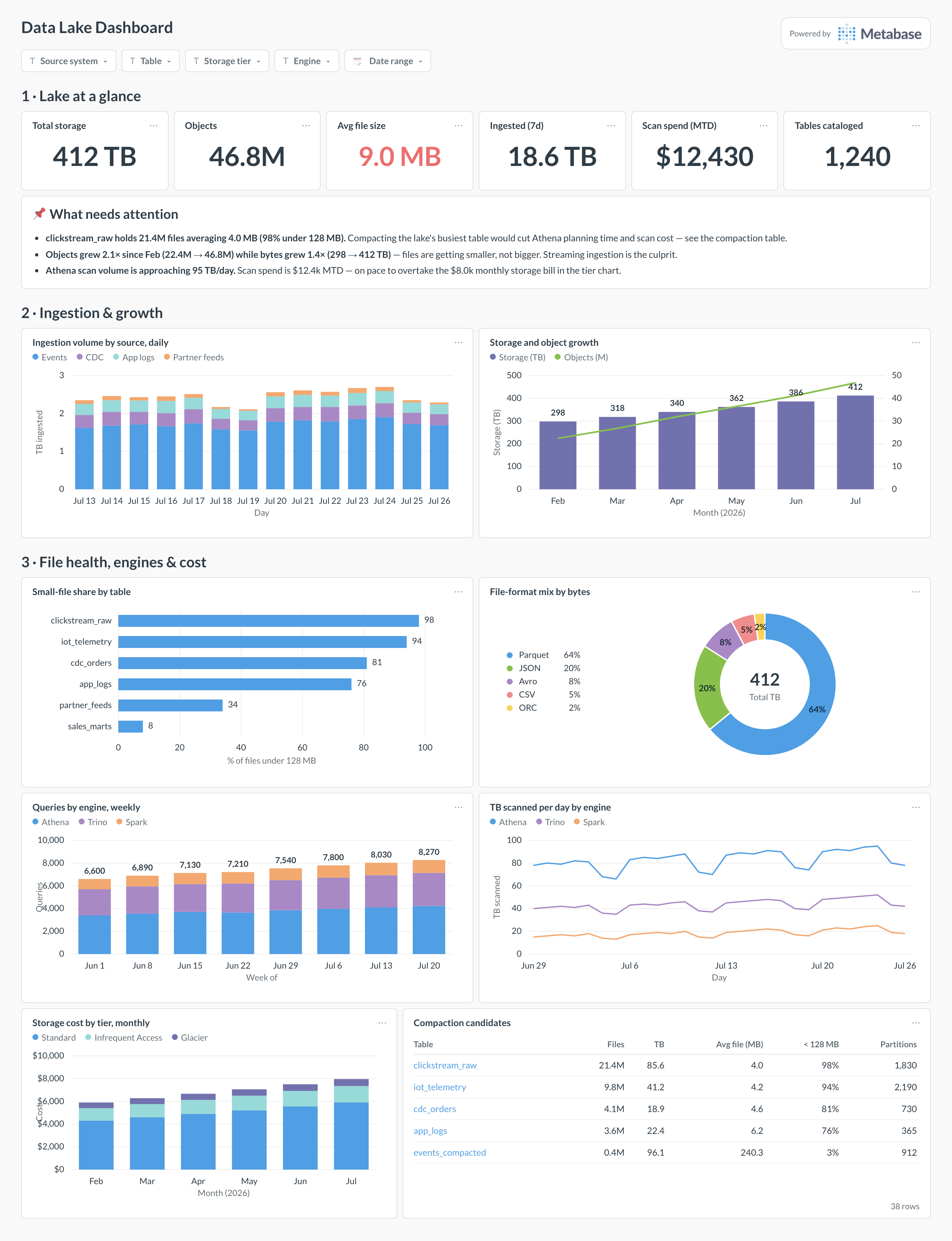
Here’s the layout this guide builds. Headline size, object, and spend figures sit at the top next to an attention card that names the worst offenders; ingestion and growth trends come next, because most lake problems arrive with the data; file health, engine usage, and tier costs sit at the bottom for the optimization work.
Which cards belong on a data lake dashboard?
The eight below cover intake, growth, file health, and cost — the four ways a lake quietly turns into a swamp.
- Ingestion volume by source, daily (stacked bar)
- Storage and object growth, monthly — TB as bars, object count as a line (combo)
- Small-file share by table — percent of files under 128 MB (row)
- File-format mix — Parquet, ORC, Avro, JSON, CSV (donut)
- Queries by engine, weekly (stacked bar)
- TB scanned per day by engine (line)
- Storage cost by tier, monthly (stacked bar)
- Compaction candidates — tables ranked by file count and average file size (table)
What data does the dashboard need?
- Object-store inventory — key, size, storage class, and last-modified per object, delivered daily (S3 Inventory, GCS Storage Insights, or Azure blob inventory).
- Catalog metadata — tables and partition keys from Glue or the Hive metastore, or a table format’s own
filesandpartitionsmetadata tables. - Engine query logs — bytes scanned, runtime, and engine from Athena workgroup metrics, a Trino event listener, or Spark event logs.
- Billing data for storage by tier and per-TB scan charges, so cost cards show dollars rather than bytes.
- A daily rollup per table — file count, total bytes, average file size, small-file share, and partition count computed from the inventory.
How do you build it?
- Turn on object-store inventory delivery to a reporting prefix and register it in the catalog, so the inventory itself is queryable as a table.
- Land engine query logs next to it — Athena’s per-workgroup metrics and a Trino event listener both write structured records with bytes scanned per query.
- Build a daily rollup per table: file count, bytes, average file size, share of files under 128 MB, and partition count — plus a per-source ingestion delta from consecutive snapshots.
- Connect the engine to Metabase (see the Athena or Presto/Trino guides) and point every card at the rollups, never the raw inventory.
- Add filters for source system, table, storage tier, engine, and date range, then subscribe the platform channel to a weekly snapshot.
Example card SQL
SELECT
i.table_name,
COUNT(*)                                              AS files,
ROUND(SUM(i.size_bytes) / POWER(1024, 4), 2)          AS tb,
ROUND(AVG(i.size_bytes) / POWER(1024, 2), 1)          AS avg_file_mb,
ROUND(100.0 * SUM(CASE WHEN i.size_bytes < 128 * 1024 * 1024
                       THEN 1 ELSE 0 END) / COUNT(*), 1)
                                                      AS small_file_pct,
COUNT(DISTINCT i.partition_key)                       AS partitions
FROM lake_reporting.object_inventory i
WHERE i.snapshot_date = CURRENT_DATE - INTERVAL '1' DAY
GROUP BY i.table_name
HAVING AVG(i.size_bytes) < 128 * 1024 * 1024
ORDER BY files DESC
LIMIT 20;
Related
Metrics
Integrations
Dashboards
FAQ
What is a data lake dashboard?
How is this different from a data warehouse dashboard?
Why do small files matter so much?
How does Metabase query a data lake?
How do I measure ingestion volume by source?
source/table/partition prefix convention pays off. Or pipeline metadata — your ingestion tool's own run logs record rows and bytes written per sync. The inventory delta is authoritative (it catches writers that bypass the pipeline); the pipeline numbers explain intent. When the two disagree, something is writing to the lake that shouldn't be — worth a card of its own once it has happened to you.What should I do about storage tiers?
Do Iceberg, Delta, or Hudi change this dashboard?
files and partitions, Delta's DESCRIBE DETAIL — so the small-file and partition-growth cards become simple SQL instead of inventory crunching. The problems themselves remain: streaming writes still produce small files (now plus snapshot and manifest debt), and compaction still has to run. Add a card for snapshot count or oldest unexpired snapshot per table; unbounded metadata growth is the table-format-specific failure mode.