





What does an attack surface coverage dashboard show in Metabase?
An attack surface coverage dashboard shows whether your scanners and sensors actually see everything: scan coverage by asset group, EDR deployment, assets nobody has scanned in 30 days, and the unknowns discovered this week. It's built from inventory and scan data synced from tools such as Tenable, CrowdStrike, Wiz, and Orca Security.
For: security engineers, infrastructure teams, and CISOs. Grain: one row per asset, joined to its latest scan and sensor check-in.
What does an attack surface coverage dashboard look like?
Here’s the layout this guide builds, at the grain of a single asset: how much of the inventory is actually scanned and sensored, which asset classes and teams the gaps sit in, and how fast new assets are appearing. Read it before you trust any vulnerability count, because coverage sets that count’s denominator.
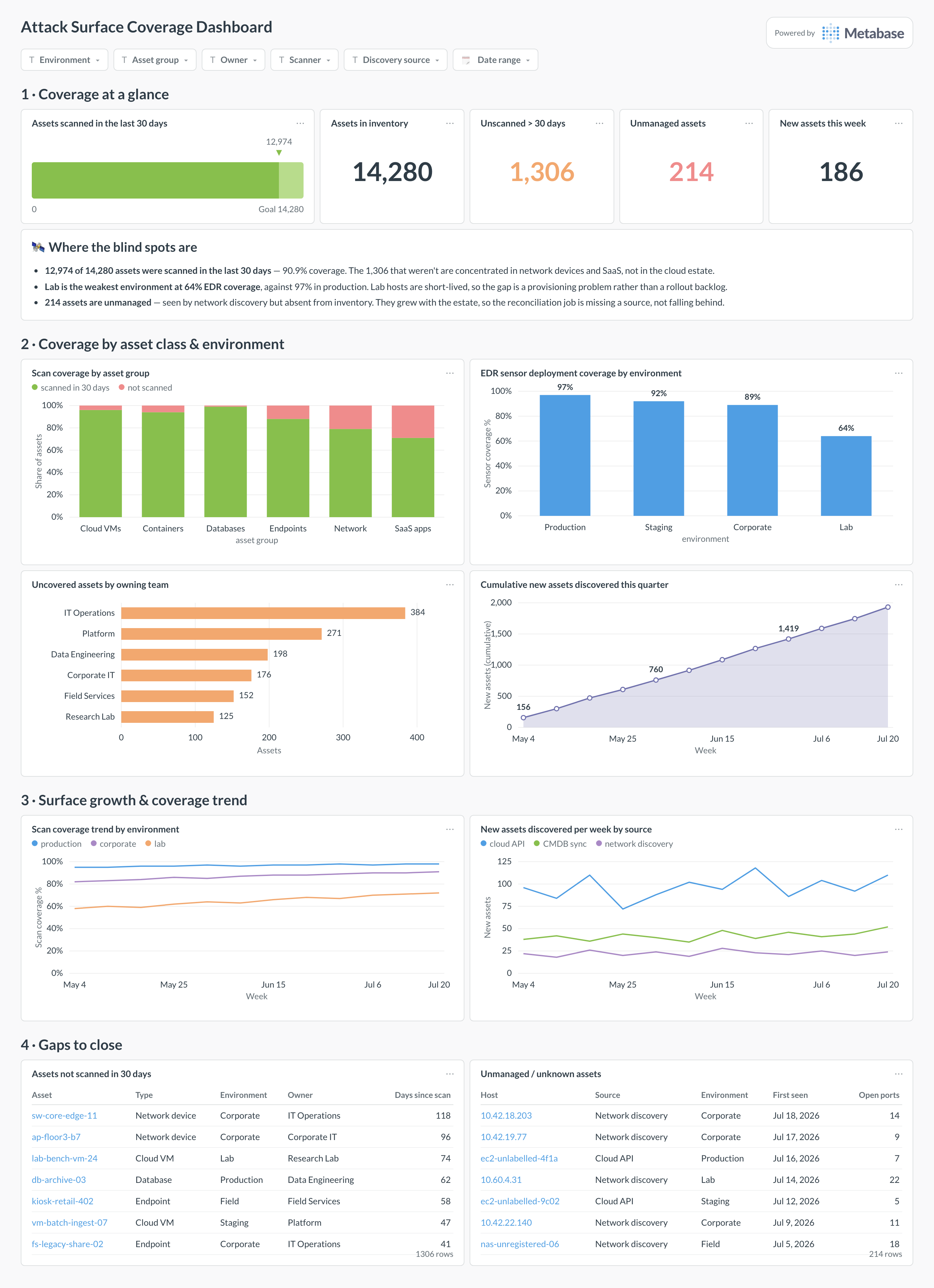
An example attack surface coverage dashboard in Metabase, built from Tenable, CrowdStrike, and Wiz data. Figures are illustrative.
Which cards belong on an attack surface coverage dashboard?
- Scan coverage by asset group (bar)
- EDR sensor deployment coverage by environment (bar)
- Assets not scanned in 30 days with owner (table)
- New assets discovered per week by source (line)
- Unmanaged / unknown assets — seen by discovery, absent from inventory (table)
- Coverage trend over time by environment (line)
What data does the dashboard need?
assets— the authoritative inventory, with source,first_seen, environment, and status.scan_events— asset, scanner, andlast_scanned_at.sensor_inventory— EDR sensor install and last check-in per host.
How do you build it?
- Build the inventory by reconciling independent sources — cloud APIs, the CMDB, and scanner discovery — so the denominator isn’t just what the scanner already sees.
- Join each asset to its most recent scan and sensor check-in, keeping scan and agent coverage as separate facts.
- Classify never-seen-recently assets as stale or decommissioned using liveness signals, so dead machines leave the denominator.
- Build the coverage-by-group bar and unscanned-assets table first; add discovery trends and unmanaged-asset views next.
Example card SQL
SELECT
  a.asset_group,
  COUNT(*) AS total_assets,
  COUNT(*) FILTER (
    WHERE s.last_scanned_at >= CURRENT_DATE - INTERVAL '30 days'
  ) AS scanned_last_30d,
  ROUND(
    100.0 * COUNT(*) FILTER (
      WHERE s.last_scanned_at >= CURRENT_DATE - INTERVAL '30 days'
    ) / NULLIF(COUNT(*), 0), 1
  ) AS coverage_pct
FROM assets a
LEFT JOIN (
  SELECT asset_id, MAX(last_scanned_at) AS last_scanned_at
  FROM scan_events
  GROUP BY asset_id
) s ON s.asset_id = a.asset_id
WHERE a.status = 'active'
GROUP BY a.asset_group
ORDER BY coverage_pct ASC;
Related
Metrics
Integrations
Dashboards
FAQ
What is an attack surface coverage dashboard?
What's the denominator problem in coverage metrics?
assets by reconciling independent sources — cloud provider APIs, the CMDB, and scanner discovery — and treat assets that appear in only one source as the interesting rows. The unmanaged-assets card exists precisely to surface what the scanners alone would never admit is missing.