




What is scan coverage, and how do you measure it in Metabase?
Scan coverage is the share of your asset inventory that was scanned — or protected by a healthy agent — within a defined window. It's the denominator check for every other vulnerability metric: an open criticals count only describes the assets you actually scan. Measure it in Metabase by joining scan telemetry from Tenable, CrowdStrike, SentinelOne, or Orca Security against an inventory reconciled from cloud APIs and your CMDB — not from the scanner itself.
assets scanned in window ÷ total inventory, by asset group. The whole metric lives or dies on the denominator: an inventory sourced from the scanner itself trends toward 100% by construction. What does a scan coverage chart look like in Metabase?
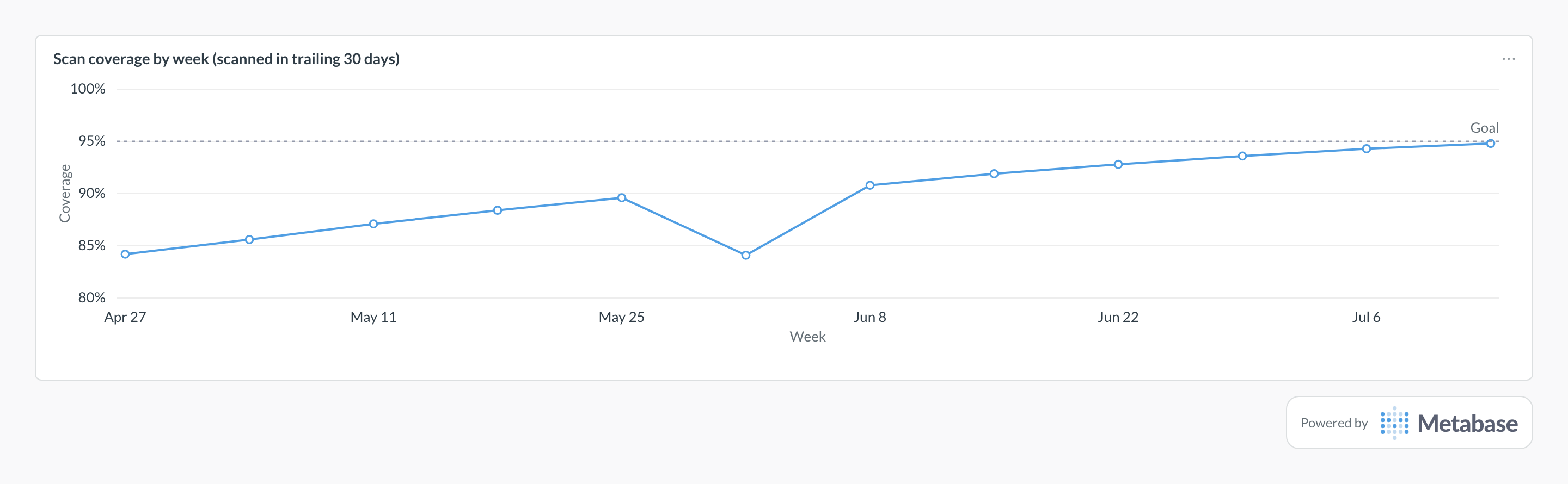
Chart the share of the reconciled inventory scanned in the trailing 30 days, week by week, against the coverage target: the climb from about 84% toward the 95% goal is scanner rollout and agent fixes landing. A dip like the week of Jun 1’s usually means reconciliation just discovered assets the scanner had never seen — the denominator got honest, which is the metric doing its job.
What scan coverage measures
It measures how much of your estate your vulnerability data can even see. Zero findings on an asset group can mean it’s clean or that it’s never been scanned — coverage is what distinguishes the two. That makes it the honesty check that comes before remediation speed or SLA compliance: those metrics only apply to findings that exist, and findings only exist where scanning happens. The gap list — known to the cloud API, never seen by the scanner — is where breaches like to start.
What data does it need?
- A reconciled
assetstable built from independent sources — cloud provider APIs, CMDB, agentless discovery — withstatus,asset_group, anddiscovery_source. - Scan and agent telemetry joined onto it as
last_scanned_at(or last healthy agent check-in). - Lifecycle data so decommissioned assets leave the denominator instead of lingering as “unscanned.”
- Per-asset-class window definitions — servers, internet-facing hosts, and ephemeral infrastructure all need different ones.
SQL patterns
-- assets: inventory reconciled from cloud APIs / CMDB,
-- not just what the scanner already knows about
SELECT
  a.asset_group,
  COUNT(*) AS inventory,
  COUNT(*) FILTER (
    WHERE a.last_scanned_at >= CURRENT_DATE - INTERVAL '30 days'
  ) AS scanned_30d,
  ROUND(
    100.0 * COUNT(*) FILTER (
      WHERE a.last_scanned_at >= CURRENT_DATE - INTERVAL '30 days'
    ) / NULLIF(COUNT(*), 0), 1
  ) AS coverage_pct
FROM assets a
WHERE a.status = 'active'
GROUP BY 1
ORDER BY coverage_pct;SELECT
a.hostname,
a.asset_group,
a.discovery_source, -- how we know it exists: cloud API, CMDB, scanner
a.first_discovered_at::date AS discovered,
a.last_scanned_at::date AS last_scanned
FROM assets a
WHERE a.status = 'active'
AND (
a.last_scanned_at IS NULL
OR a.last_scanned_at < CURRENT_DATE - INTERVAL '30 days'
)
ORDER BY a.last_scanned_at ASC NULLS FIRST;Pitfalls
Where this metric applies
- Tenable + Metabase — scan history and last-seen timestamps per asset
- CrowdStrike + Metabase — sensor deployment and health across hosts
- SentinelOne + Metabase — agent check-ins and version status
- Orca Security + Metabase — agentless discovery of cloud workloads
Related
Metrics
Dashboards
FAQ
Where should the asset inventory come from?
What scan window should we use?
INTERVAL for everything.Does an installed agent count as covered?
How do you calculate scan coverage?
scanned_in_window / inventory, grouped by asset group. Scope the denominator to active assets — decommissioned machines still in the CMDB shouldn't count as unscanned — and keep the never-scanned and stale lists as the operational follow-up.How do you track scan coverage in Metabase?
assets table from cloud APIs and your CMDB, then join scan and agent telemetry from Tenable, CrowdStrike, SentinelOne, or Orca Security to stamp last_scanned_at. Chart coverage by asset group, keep the never-scanned list with discovery source as the work queue, and read it next to open critical vulnerabilities on an attack surface coverage dashboard — findings only exist where scanning happens.